Allocation over ETF returns

examples/allocation_etfs.py runs keeks’ allocation layer over a real six-ETF book — SPY, QQQ, IWM, TLT, GLD and VNQ, spanning US large-cap and small-cap equities, growth, long treasuries, gold and real estate — and asks the question the single-bet pages cannot: what do the allocators actually disagree about, when they all size the same portfolio?

Two joint-return models are built from the same committed daily simple returns (examples/data/etf_returns.csv, window 2022-10-03 to 2025-10-01): the empirical bootstrap via keeks.allocation.models.scenario_model(), and per-option Student-t marginals fitted by maximum likelihood via keeks.allocation.models.fit_marginals_model() (a scipy-gated extra). Each model is then replayed for 1,000 periods through the keeks.allocation.simulators.AllocationSimulator with seven books side by side: five allocators — MeanVariance at λ = 1, RiskBudgeting (ERC), HierarchicalRiskParity, MeanCVaR at α = 5% and the online ExponentialGradient — against two benchmarks, equal weight and global minimum variance. Every allocator inside a pass meets the same seeded realizations (common random numbers, seed 20260803), so the comparison is the allocators’ and not the draw luck’s.

Warning

These are simulated results from a model, not a forecast and not investment advice. The replay resamples one three-year window of history and charges no fees — neither of which holds in a real book. Keeks is an educational library; treat every number below as a property of the model, not a prediction about money.

Growth paths

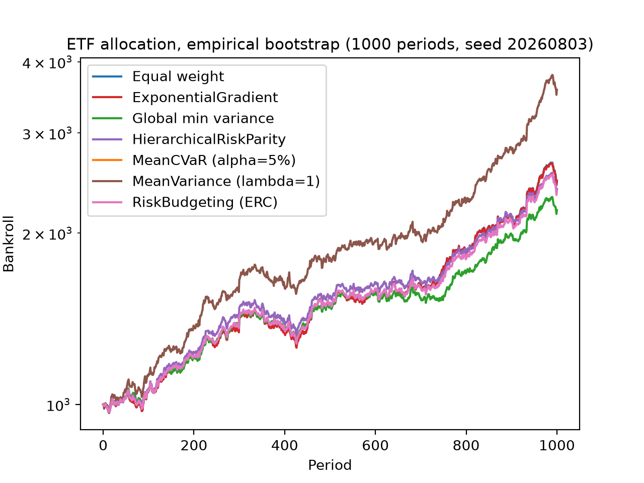
Growth of the seven books under the empirical bootstrap model, seed 20260803. MeanVariance at λ = 1 leads throughout; MeanCVaR’s flat line is its unit-risk-aversion posture holding cash (below).

The same comparison under fitted fat-tailed marginals keeps the ordering:

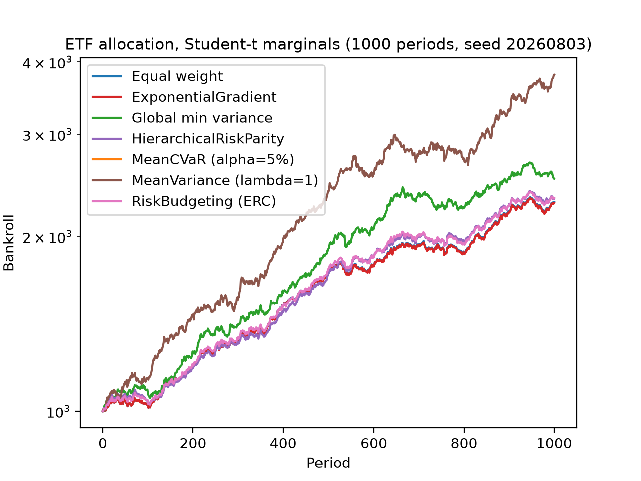
Growth of the same seven books under Student-t marginals fitted to the same window. The Student-t draws carry no scenario rows, so MeanCVaR — still bound to the empirical scenarios — reprices nothing here.

Drawdown and weights

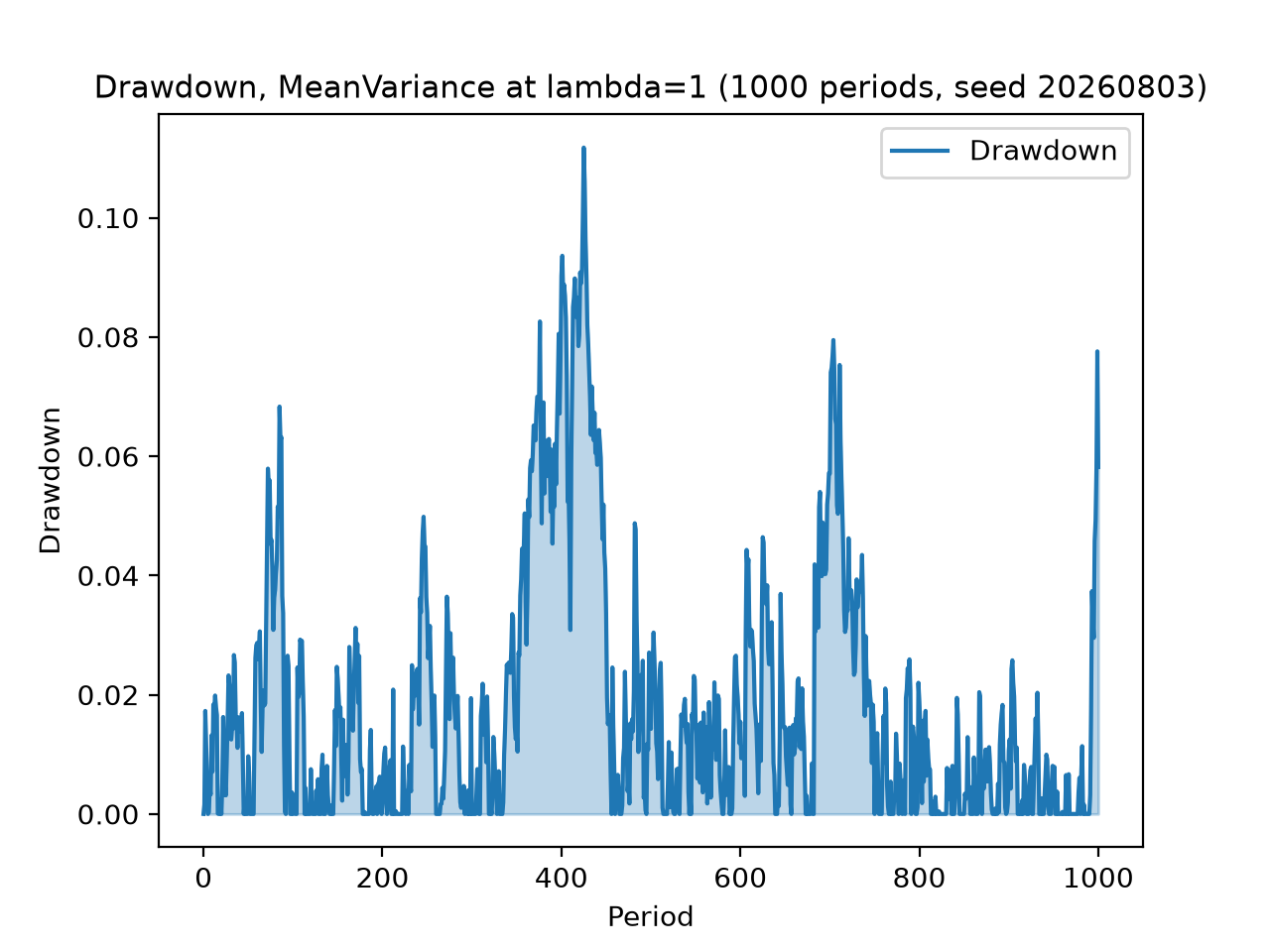
Peak-to-trough drawdown of the leading book, MeanVariance at λ = 1, over the empirical-bootstrap replay. The growth story above is bought with drawdowns of this size.

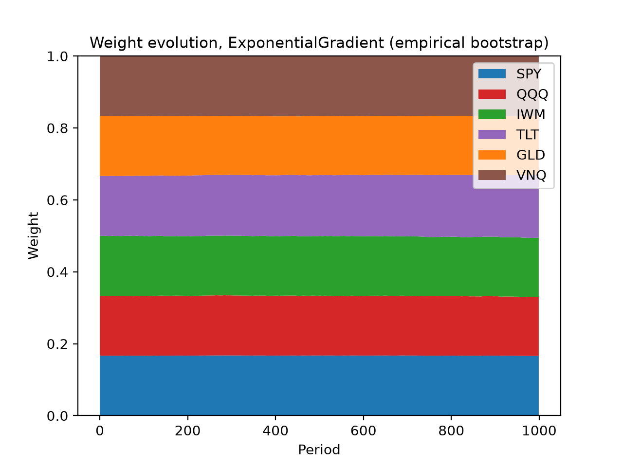
Weight evolution of the online allocator, ExponentialGradient, recorded each period during the empirical-bootstrap pass and relabelled with the tickers. It starts near equal weight and barely moves.

MeanCVaR holds cash, on purpose

The flat line at $1,000 in both growth charts is MeanCVaR at its shipped unit risk aversion, and it is the example’s most instructive result rather than a failed solve. The objective trades expected return against the tail’s expected loss one-for-one, and it is positively homogeneous in the return scale — so on daily-frequency market data, where expected daily return sits far below the tail’s expected loss, the honest optimum is full cash. No unit choice changes that; the risk-aversion dial is a documented follow-up. The mean-variance family, which squares the same trade-off against variance rather than the tail, sizes aggressively on the same inputs — which is exactly the contrast the side-by-side replay exists to show.

Reproducing it

One command, from a checkout of the repository:

uv run python examples/allocation_etfs.py

The default run is fully offline — it loads the committed fixture, whose provenance header names the tickers, the date window and the refresh command — and prints a comparison table (final funds, growth, per-period volatility, maximum drawdown) for each pass before writing the four charts above into examples/output/. Pass --refresh to re-download the window from Yahoo Finance via yfinance (a development-only dependency; keeks never imports it at runtime) and rewrite the fixture first.