The St. Petersburg paradox
Flip a fair coin until it lands tails and you are paid $2n, where n is the number of flips. Each branch of the game contributes (1/2n) × 2n = $1 to the expectation, so the expected payout is infinite — and yet no rational person pays much to play. That gap between infinite expectation and finite willingness-to-pay is the St. Petersburg paradox, and it is the cleanest demonstration of why a growth criterion, not an expectation, is what sizes a bet.
examples/st_petersburg_paradox.py turns the paradox into a pricing
question for keeks’ strategies: what is the maximum entry price each of
the nine shipped strategies would pay to play one round, at bankrolls of
$1, $10, $100 and $1,000? Each strategy answers through
calculate_max_entry_price over the game’s outcome distribution, capped
at 1,000 flips (the practical limit of float64), where the capped game’s
expected value is $1,000 — each flip contributing exactly $1 of it.
Warning
These are simulated results from a model, not a forecast and not investment advice. The game is a mathematical ideal — a fair coin, an unlimited counterparty, and a payout schedule no real venue honours — and the entry prices are what each rule would bid inside its own assumptions. Keeks is an educational library; treat every number below as a property of the model, not a prediction about money.
What the spread says
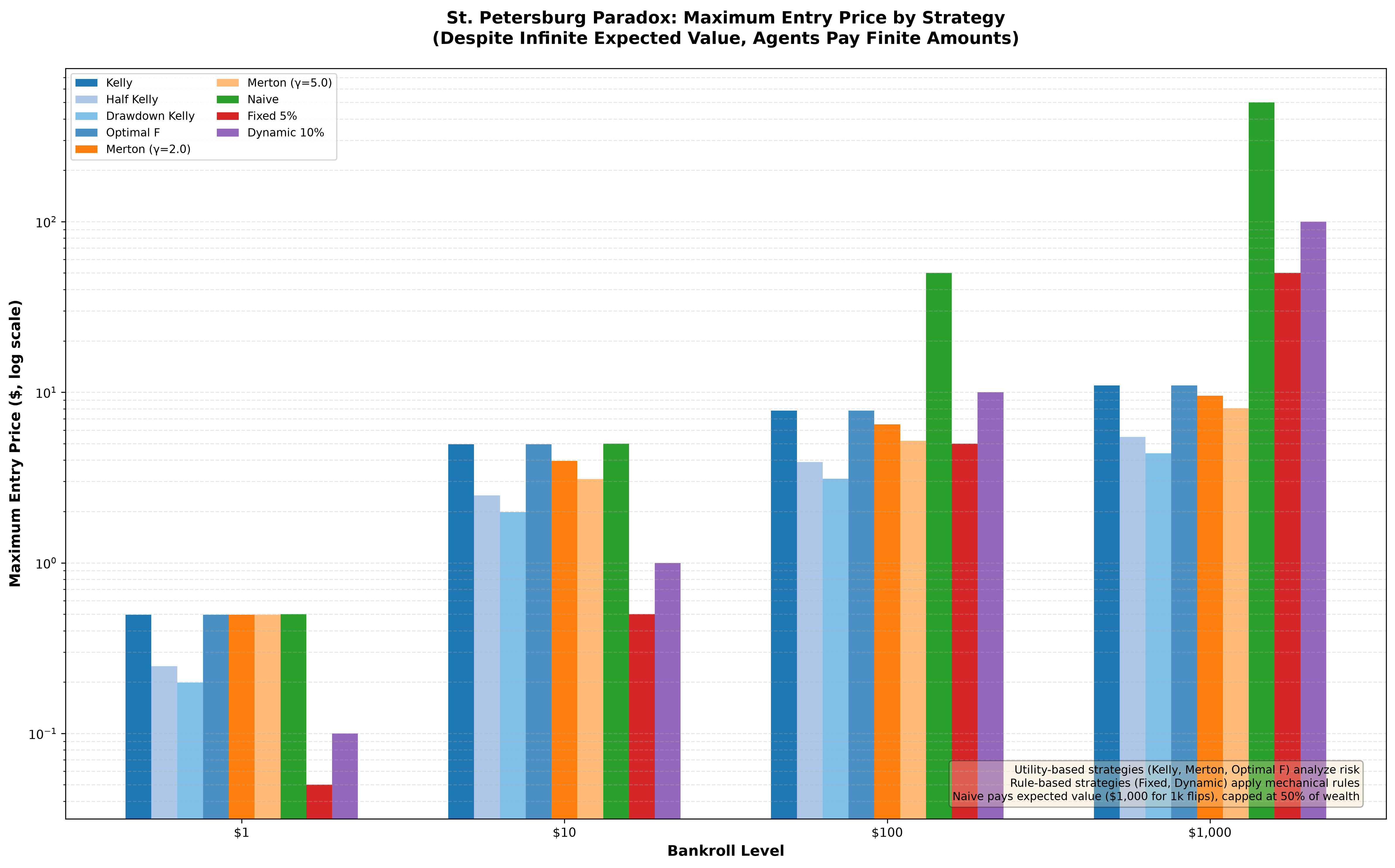
Maximum entry price by strategy and wealth level. Higher bars mean the rule would pay more for one round of a game with infinite expected value.
The utility-based rules — Kelly, its fractional and drawdown-adjusted variants, Optimal F, and the Merton shares at risk aversion 2 and 5 — price the game conservatively and scale gently with wealth: log and power utility refuse to pay much for lottery-like tails, whatever the expectation says. The rule-based strategies bid mechanically, and at a $1,000 bankroll they are the aggressive bidders: Dynamic 10% bids about $100, Fixed 5% bids a wealth fraction, and Naive pays the capped expected value — 50% of wealth, about $460, the tallest bar on the chart. Four orders of magnitude separate the most and least willing bidders, all facing the same infinite-EV game.
That inversion — the “naive” rule outbidding Kelly for a positive-EV game — is the paradox made practical: an expectation-only rule cannot see that the payout is concentrated in a branch you will essentially never see, while a growth criterion prices the bet you actually experience.
Reproducing it
One command, from a checkout of the repository:
uv run python examples/st_petersburg_paradox.py
It prints the maximum entry price for each of the nine strategies at each
wealth level — in dollars and as a percentage of bankroll — and writes the
chart plus examples/output/st_petersburg_paradox.csv with both views
of every cell.